The concept of work done is an integral part of classical physics, particularly because of something called the 'work-energy principle'.
In this post, I will formally define work done, show how (in some situations, where the forces and paths we are considering are sufficiently 'nice'), it can be computed.
First lets define work done in the case of a constant force and motion in a straight line.
$\displaystyle Definition \ 1 \ (Work \ done \ (under \ constraints) ) - $ The work done by a constant force $\vec{F}$ acting on an object that is displaced $\vec{s}$ is $\vec{F} \cdot \vec{s}$
Describing the above definition using only English, we may write ' The work done by a constant force acting on an object is equal to the signed product of the magnitude of the objects displacement in the direction of the force multiplied by the magnitude of the force' , where the sign depends only on whether or not the component of the objects displacement along the line of the force vector points in line with the direction of the force or opposite the direction of the force.
Here is a diagram to illustrate this:
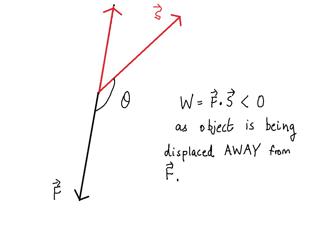
$\square$
Now lets consider a more complicated example. What if an object is moving in some arbitrary force field (you can think of this as a region of space where at every single point within the specified region, a force is acting in some direction), where the force in question may be of variable magnitude. Furthermore, the object need not be moving in a straight line.
Lets draw another picture to illustrate this:

The picture I above, admittedly, is a bit overkill. Although drawing all those arrows in MS paint felt therapeutic, my artistic release didn't end up producing a vector field that appeared very continuous. Nonetheless, the point of the image was to show how far away we can deviate from the case where there is only a constant force acting on an object.
So the natural question now becomes, how do we compute the work done by a force on an object in this more general case?
$\square$
Lets make a few assumptions in order to answer this question. First of all, suppose are force is $\displaystyle \vec{F} : E \subset \mathbb{R}^k \mapsto \mathbb{R}^k$. Lets also assume our force is continuous on $E$.
Lets say the path were moving in, from $t=a$ to $t=b$ is $\vec{\gamma} : [a,b] \mapsto E $. Furthermore, we'll assume this path is continuously differentiable.
Here's another (poorly drawn) picture to illustrate this:

Now, in the picture above, I've divided the curve $\displaystyle \vec{\gamma}$ into segments.
This division actually corresponds to a partition of time, $\{t_0 = a, t_1, t_2, ... , t_{n-1},t_n=b\}$.
Assuming our force is continuous, and the intervals of time we have created in our partition are small enough, it is reasonable to believe the force $\vec{F}$ acting on the object moving in $\vec{\gamma}$ is approximately constant in magnitude and direction throughout the entire interval $[t_{i-1},t_i]$ for any $i \in \{1,2,....,n\}$.
Therefore, within such an interval of time, we can approximate the total work done by this force on the object moving throughout $[t_{i-1}, t_i]$ as $\displaystyle \vec{F}(\vec{\gamma}(t_{i*})) \cdot (\vec{\gamma}(t_i) - \vec{\gamma}(t_{i-1}))$, where $t_{i*}$ is any point in $[t_{i-1}, t_i]$.
Now, since were not only moving in the curve $\vec{\gamma}$ during a specific interval $[t_{i-1},t_i]$, but throughout the whole of $[a,b]$, we need to account for the work this force is doing on us during all other intervals of time as well. This is why we take a summation:
$\displaystyle \sum_{i=1}^n \vec{F}(\vec{\gamma}(t_{i*})) \cdot (\vec{\gamma}(t_i) - \vec{\gamma}(t_{i-1})) $ and call this our first approximation of work done on the object moving in $\displaystyle \vec{\gamma}$ from $t=a$ to $t=b$. In the picture above, $\triangle \vec{\gamma}(t_i) = \vec{\gamma}(t_i) - \vec{\gamma}(t_{i-1})$ .
$\square$
In mathematics, while first approximations are always appreciated, one is usually interested in formulating better, more accurate approximations in order to better capture what is really going on.
In the previous illustration, we partitioned the interval of time the object being considered was moving within, into $n$ sub-intervals: $[t_{i-1},t_i]$ from $i=1$ to $i=n$. Within each of these sub-intervals, we assumed that the particle was moving in a straight line from $\displaystyle \vec{\gamma}(t_{i-1})$ to $\displaystyle \vec{\gamma}(t_i)$ and that the force acting on the object during this interval of time was constant in direction and magnitude, and given by $\vec{F}(\vec{\gamma}(t_{i*}))$ where $t_{i*}$ is some point in $[t_{i-1},t_i]$.
This doesn't capture exactly what is going on though, as it could be that even during this very small interval of time, the object is moving like this:

We immediately see that our approximation of the objects path is a gross under-approximation, and therefore, we also see that it doesn't even appear that the force we are interested in is relatively constant throughout the interval of time we have chosen! This is an unhappy state of affairs, and in an effort to rectify this, we will further subdivide our interval of time $[t_{i-1},t_i]$ so as to better capture what is really going on:

Ahh.. much better.
$\square$
So we have figured out a way to produce better approximations, all we need to do is simply subdivide our interval of time $[a,b]$ into finer and finer sub-intervals, as the finer we partition, the better we capture whats going on within these intervals of time.
It thus makes sense to define work done as $\displaystyle \lim_{||P|| \to 0} \sum_{i=1}^n \vec{F}(\vec{\gamma}(t_{i*})) \cdot (\vec{\gamma}(t_i) - \vec{\gamma}(t_{i-1})) $, where $\displaystyle ||P|| = max(t_i - t_{i-1})$ where $i = \{1,2,...,n\}$, granted this limit exists.
All this means is, that work done can be defined as the limit of the sum of approximations to work done over sub-intervals of our entire interval of time, $[a,b]$, as the length of these sub-intervals gets smaller and smaller.
Although we now have a definition of work done, at the present moment, it doesn't seem to be very illuminating, as we have no idea how we can actually compute such a thing!
As it turns out, given we make some reasonable assumptions about $\vec{F}$ and $\vec{\gamma}$, $\displaystyle \lim_{||P|| \to 0} \sum_{i=1}^n \vec{F}(\vec{\gamma}(t_{i*})) \cdot (\vec{\gamma}(t_i) - \vec{\gamma}(t_{i-1})) $ isn't very difficult to compute.
The assumptions we will make are, that
(1) $\vec{\gamma} : [a,b] \mapsto E \subset \mathbb{R}^m$ is continuously differentiable on $[a,b]$
(2) $\vec{F} : E \mapsto \mathbb{R}^m$ is continuous on $E$
(Note: The definition of the term 'continuously differentiable' is as follows: If $f$ is continuously differentiable on a set $A$, $f'$ is continuous on $A$)
The best way to think of a continuously differentiable function is as 'smooth'. The function must have no sharp corners, and no holes, furthermore the functions 'velocity', or rate of growth, may not become arbitrarily large in a finite interval of time/space.
This rules out some functions, for example, a particle moving with position
$ \frac{-1}{t}$ has arbitrarily large speed at some point in any interval $(0,t]$, in fact, it can even have arbitrarily large average speed in an interval of the form $(0,t]$.
Although, as long as we only consider the function on intervals $[x,y]$ with $x>0$, the function is indeed continuously differentiable.
$\square$
Now, using assumptions (1) and (2), we will prove that $\displaystyle \lim_{||P|| \to 0} \sum_{i=1}^n \vec{F}(\vec{\gamma}(t_{i*})) \cdot (\vec{\gamma}(t_i) - \vec{\gamma}(t_{i-1})) = \int_{a}^b \vec{F}(t) \cdot \vec{\gamma'}(t) dt $
I will present a rigorous proof first, and then a tl;dr 'proof' of this.
One thing to note when reading this proof is that when a letter is used in some context, for example, the letter $m$ in $\mathbb{R}^m$, if such a letter is then re-used further down the proof, the reader should immediately assume that the letter being used further down has exactly the same meaning as when it was first used.
Since $\vec{\gamma}'(t)$ is continuous on $[a,b]$, it's component functions must be continuous on $[a,b]$.
We also know that $\vec{\gamma}' : [a,b] \mapsto \mathbb{R}^m$
Therefore, with respect to the standard basis $\{\vec{u_1},\vec{u_2}, ... ,\vec{u_m}\}$, we know that $\displaystyle \vec{\gamma}'(t) = \sum_{k=1}^m {\gamma'_k}(t)\vec{u_k} $
Furthermore, each component function ${\gamma'_k}(t)$ is also uniformly continuous on $[a,b]$ (by continuity on a closed interval of $\mathbb{R}$ implies uniform continuity on the same interval)
Lets now consider the function $\vec{F}(\vec{\gamma}) : [a,b] \mapsto \mathbb{R}^m$. By assumption (2), this is continuous on $[a,b]$.
Therefore $|\vec{F}(\vec{\gamma})| : [a,b] \mapsto \mathbb{R}$ is a real valued function that is continuous on the interval $[a,b]$. As a consequence, by boundedness of real valued functions that are continuous on a closed interval, we know that there exists a real number $M > 0$ such that $|\vec{F}(\vec{\gamma}(t))| < M$ for all $t \in [a,b]$.
Therefore there must exist a $\delta >0$ such that for any partition $P = \{t_0=a,t_1,...,t_{n-1},t_n=b\}$ if $||P|| < \delta$, we can ensure that for any $x,y \in [t_{i-1},t_i]$, $\displaystyle |{\gamma'_k}(x) - {\gamma'_k}(y)| < \frac{\epsilon}{mM(b-a)}$
Lets assume we've chosen a partition $P$ of $[a,b]$ with $||P|| < \delta$ so that $\displaystyle |{\gamma'_k}(x) - {\gamma'_k}(y)| < \frac{\epsilon}{mM(b-a)}$ for all $k \in \{1,2,....,m\}$.
Now, consider $ (\vec{\gamma}(t_i) - \vec{\gamma}(t_{i-1}))$
We know that for any sub-interval $[t_{i-1},t_i]$ of $P$, $(\vec{\gamma}(t_i) - \vec{\gamma}(t_{i-1})) = \sum_{k=1}^m ({\gamma_k}(t_i) - {\gamma_k}(t_{i-1}))\vec{u_k}$
By the mean-value theorem, for any interval $[t_{i-1},t_i]$, there exists a $p_k \in [t_{i-1},t_i]$ such that ${\gamma_k}(t_i) - {\gamma_k}(t_{i-1}) = {\gamma'_k}(p_k) (t_i - t_{i-1})$
Therefore, $\displaystyle (\vec{\gamma}(t_i) - \vec{\gamma}(t_{i-1})) = \sum_{k=1}^m ({\gamma_k}(t_i) - {\gamma_k}(t_{i-1}))\vec{u_k} = \sum_{k=1}^m {\gamma'_k}(p_k) (t_i - t_{i-1}) \vec{u_k}$
Now, as we have chosen $||P|| < \delta$, and each $p_k \in [t_{i-1},t_i]$, we know that
$\displaystyle |\sum_{k=1}^m {\gamma'_k}(p_k) (t_i - t_{i-1}) \vec{u_k} - \sum_{k=1}^m {\gamma'_k}(t_i*) (t_i - t_{i-1}) \vec{u_k}| < \sum_{k=1}^m |{\gamma'_k}(p_k) - {\gamma'_k}(t_i*)| (t_i - t_{i-1}) < \frac{\epsilon}{M(b-a)} (t_i - t_{i-1})$
But $\displaystyle \sum_{k=1}^m {\gamma'_k}(p_k) (t_i - t_{i-1}) \vec{u_k} = (\vec{\gamma}(t_i) - \vec{\gamma}(t_{i-1}))$ and $\displaystyle \sum_{k=1}^m {\gamma'_k}(t_i*) (t_i - t_{i-1}) \vec{u_k}| = \vec{\gamma'}(t_i*) (t_i - t_{i-1})$
Therefore, for any interval $[t_{i-1},t_i]$, $|(\vec{\gamma}(t_i) - \vec{\gamma}(t_{i-1})) - \vec{\gamma'}(t_i*) (t_i - t_{i-1})| < \frac{\epsilon}{M(b-a)} (t_i - t_{i-1})$
Now, lets consider $\displaystyle \sum_{i=1}^n \vec{F}(\vec{\gamma}(t_{i*})) \cdot (\vec{\gamma}(t_i) - \vec{\gamma}(t_{i-1})) $
Note that $\displaystyle | \sum_{i=1}^n \vec{F}(\vec{\gamma}(t_{i*})) \cdot (\vec{\gamma}(t_i) - \vec{\gamma}(t_{i-1})) - \sum_{i=1}^n \vec{F}(\vec{\gamma}(t_{i*})) \cdot \vec{\gamma'}(t_i*) (t_i - t_{i-1}) | \leq \sum_{i=1}^n |\vec{F}(\vec{\gamma}(t_{i*}))| |(\vec{\gamma}(t_i) - \vec{\gamma}(t_{i-1})) - \vec{\gamma'}(t_i*) (t_i - t_{i-1})|$
by the Cauchy-Schwarz and Triangle inequalities.
But $\displaystyle \sum_{i=1}^n |\vec{F}(\vec{\gamma}(t_{i*}))| |(\vec{\gamma}(t_i) - \vec{\gamma}(t_{i-1})) - \vec{\gamma'}(t_i*) (t_i - t_{i-1})| < \sum_{i=1}^n M |(\vec{\gamma}(t_i) - \vec{\gamma}(t_{i-1})) - \vec{\gamma'}(t_i*) (t_i - t_{i-1})| < \sum_{i=1}^n \frac{\epsilon}{(b-a)} (t_i - t_{i-1}) < \epsilon $
This shows that given $||P||$ is sufficiently small, our 'approximation' for work done:
(3) $\displaystyle \sum_{i=1}^n \vec{F}(\vec{\gamma}(t_{i*})) \cdot (\vec{\gamma}(t_i) - \vec{\gamma}(t_{i-1})) $
can be made arbitrarily close to :
(4) $\sum_{i=1}^n \vec{F}(\vec{\gamma}(t_{i*})) \cdot \vec{\gamma'}(t_i*) (t_i - t_{i-1})$
where (4) is nothing but a Riemann sum for the integral of $\vec{F}(\vec{\gamma}(t)) \cdot \vec{\gamma'}(t)$ over the interval $[a,b]$.
Due to assumptions (1) and (2), namely that $\vec{\gamma} : [a,b] \mapsto E \subset \mathbb{R}^m$ is continuously differentiable on $[a,b]$ and $\vec{F} : E \mapsto \mathbb{R}^m$ is continuous on $E$ , it follows that $\vec{F}(\vec{\gamma}(t)) \cdot \vec{\gamma'}(t)$ is
continuous on $[a,b]$, and is thus Riemann integrable.
Thus, given $||P||$ is sufficiently small, we can ensure that $\sum_{i=1}^n \vec{F}(\vec{\gamma}(t_{i*})) \cdot \vec{\gamma'}(t_i*) (t_i - t_{i-1})$
is arbitrarily close to $\displaystyle \int_{a}^b \vec{F}(t) \cdot \vec{\gamma'}(t) dt $, and thus that our approximation:
$\displaystyle \sum_{i=1}^n \vec{F}(\vec{\gamma}(t_{i*})) \cdot (\vec{\gamma}(t_i) - \vec{\gamma}(t_{i-1})) $
is also arbitrarily close to $\displaystyle \int_{a}^b \vec{F}(t) \cdot \vec{\gamma'}(t) dt $.
Thus we have proved that $\displaystyle \lim_{||P|| \to 0} \sum_{i=1}^n \vec{F}(\vec{\gamma}(t_{i*})) \cdot (\vec{\gamma}(t_i) - \vec{\gamma}(t_{i-1})) = \int_{a}^b \vec{F}(t) \cdot \vec{\gamma'}(t) dt $
$\blacksquare$
Now I will present the 'tl;dr' proof.
Most of this result actually stems from the Mean-Value-Theorem (or a slight variant of the Mean-Value-Theorem).
Essentially, the proof comes down to the fact that when the size of the sub-intervals $[t_{i-1},t_i]$ you have chosen are small, $\vec{\gamma}(t_i) - \vec{\gamma}(t_{i-1}) \approx \vec{\gamma}'(t_i*) (t_i - t_{i-1})$, where the $t_i*$ we are talking about is the same $t_i*$ in : $\sum_{i=1}^n \vec{F}(\vec{\gamma}(t_{i*})) \cdot (\vec{\gamma}(t_i) - \vec{\gamma}(t_{i-1}))$
I will illustrate why this is true when we aren't dealing with curves in $\mathbb{R}^2$ or above. That is, when the object that is moving is moving in a completely straight line, so that we don't have to concern ourselves with any 'component functions' that make things look ugly. So our object can either move 'right' $+ve$ or 'left $-ve$.
If our object is moving smoothly in a line, it's displacement from the origin may look something like this:

Now, in the figure above the point $p_i* \in (t_{i-1},t_i)$ is such that $\gamma(t_i) - \gamma(t_{i-1}) = \gamma'(p_i*) (t_i - t_{i-1})$.
Since $\gamma'$ is continuous, and the length of the interval $[t_{i-1},t_i]$ is small, we know that $\gamma'(p_i*) \approx \gamma'(t_i*)$ and therefore:
$\displaystyle \sum_{i=1}^n \vec{F}({\gamma}(t_{i*})) \cdot ({\gamma}(t_i) - \vec{\gamma}(t_{i-1})) = \sum_{i=1}^n \vec{F}({\gamma}(t_{i*})) \cdot (\gamma(p_i*)) (t_i - t_{i-1}) \approx \sum_{i=1}^n \vec{F}({\gamma}(t_{i*})) \cdot (\gamma(t_i*)) (t_i - t_{i-1})$ since all sub-intervals are small.
But $\displaystyle \sum_{i=1}^n \vec{F}({\gamma}(t_{i*})) \cdot (\gamma(t_i*)) (t_i - t_{i-1})$ is just a Riemann sum for $\displaystyle \int_{a}^b \vec{F}(t) \cdot {\gamma'}(t) dt$
The result now follows. This is also the general idea for how to go about proving this result when $\gamma$ is a vector valued function from $[a,b]$ to $\mathbb{R}^m$ when $m \geq 2$.
$\blacksquare$
In the next part of this post, I will introduce the idea of a 'conservative' force, explore the concepts of work done by gravity, gravitational potential, and the so-called 'work - energy principle'.
Thanks for reading
No comments:
Post a Comment